Equations For Motion With Constant Acceleration
Muz Play
Mar 31, 2025 · 6 min read
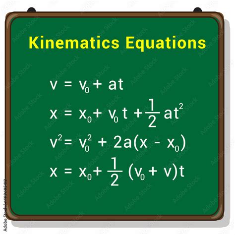
Table of Contents
Equations of Motion with Constant Acceleration: A Comprehensive Guide
Understanding motion is fundamental to physics. Whether analyzing the trajectory of a projectile, the deceleration of a car, or the freefall of an object, the equations of motion provide the mathematical framework for understanding and predicting these movements. This comprehensive guide delves into the equations of motion with constant acceleration, exploring their derivation, applications, and practical examples.
Understanding Constant Acceleration
Before diving into the equations, let's define our terms. Acceleration is the rate of change of velocity with respect to time. When acceleration is constant, it means the velocity changes by the same amount in every equal interval of time. This simplifies the analysis considerably. Imagine a car accelerating uniformly from rest; its speed increases by, say, 5 m/s every second. This represents constant acceleration. Conversely, if the car's acceleration changes—speeding up faster, then slower—then the acceleration is not constant.
The Five Key Equations
The motion of an object with constant acceleration can be completely described using five key equations. These equations relate the initial velocity (u), final velocity (v), acceleration (a), displacement (s), and time (t). Let's examine each one:
1. v = u + at
This equation relates the final velocity (v) to the initial velocity (u), acceleration (a), and time (t). It tells us how much the velocity has changed over a given time interval due to constant acceleration. This is arguably the most fundamental equation of motion.
-
Derivation: Acceleration is defined as the change in velocity divided by the change in time: a = (v - u) / t. Rearranging this equation gives us v = u + at.
-
Example: A car accelerates from rest (u = 0 m/s) at a constant rate of 2 m/s² for 5 seconds. Its final velocity (v) can be calculated as: v = 0 + (2 m/s²)(5 s) = 10 m/s.
2. s = ut + ½at²
This equation relates the displacement (s) to the initial velocity (u), acceleration (a), and time (t). It calculates how far an object travels under constant acceleration over a given time.
-
Derivation: This equation requires a bit more calculus. We start with the definition of velocity: v = ds/dt (the derivative of displacement with respect to time). Since v = u + at, we can substitute this into the equation above: ds/dt = u + at. Integrating both sides with respect to t, we arrive at s = ut + ½at².
-
Example: A ball is thrown vertically upwards with an initial velocity of 20 m/s. Ignoring air resistance and assuming an acceleration due to gravity of -9.8 m/s², we can calculate its displacement after 2 seconds: s = (20 m/s)(2 s) + ½(-9.8 m/s²)(2 s)² = 20.4 m (approximately). The negative sign indicates displacement is upwards, while acceleration is downwards.
3. v² = u² + 2as
This equation relates the final velocity (v) to the initial velocity (u), acceleration (a), and displacement (s). It's particularly useful when time is not explicitly given.
-
Derivation: This equation can be derived by eliminating time (t) from equations 1 and 2. We solve equation 1 for t: t = (v - u)/a. Substituting this value of t into equation 2 and simplifying leads to v² = u² + 2as.
-
Example: A car decelerates at a rate of -5 m/s² and comes to a stop (v = 0 m/s) after travelling 10 meters. We can calculate its initial velocity (u): 0 = u² + 2(-5 m/s²)(10 m), which gives u = 10 m/s.
4. s = [(u + v)/2]t
This equation calculates the displacement (s) using the average velocity.
-
Derivation: The average velocity is simply (u + v)/2. Since displacement is the average velocity multiplied by time, we arrive at s = [(u + v)/2]t.
-
Example: A train travels at an initial velocity of 30 m/s and then decelerates uniformly to a final velocity of 10 m/s over 10 seconds. The distance covered during this time is: s = = 200 m.
5. s = vt - ½at²
This equation is a variation of equation 2, useful when the initial velocity isn't readily available, and the final velocity is known.
-
Derivation: This can be derived by substituting v = u + at from equation 1 into equation 2 and simplifying.
-
Example: A rocket, after accelerating uniformly, reaches a final velocity of 100 m/s in 5 seconds. If its acceleration is 10m/s², how far did it travel in this time? Using the equation: s = (100 m/s)(5s) - ½(10 m/s²)(5s)² = 375m.
Choosing the Right Equation
The key to successfully solving problems involving constant acceleration lies in selecting the appropriate equation. Carefully examine the problem statement. Identify the known quantities (u, v, a, s, t) and the unknown quantity you need to find. Then, choose the equation that contains all the known and the unknown variables. This will lead you to the solution.
Practical Applications
The equations of motion with constant acceleration are not just theoretical concepts. They have numerous practical applications across various fields:
-
Engineering: Designing ramps, calculating braking distances for vehicles, analyzing projectile motion in ballistic calculations, designing roller coasters, and predicting the motion of various machines.
-
Physics: Understanding free-fall, analyzing the motion of planets (under approximations of constant gravitational acceleration), and exploring various aspects of classical mechanics.
-
Sports Science: Analyzing the trajectory of a ball in sports like baseball, basketball, and golf; calculating the ideal launch angle for maximum range or height.
-
Aerospace Engineering: Calculating launch trajectories for rockets and satellites, designing flight control systems, and analyzing the atmospheric re-entry of spacecraft.
Advanced Concepts and Considerations
While these equations work beautifully for constant acceleration, many real-world scenarios involve variable acceleration. In those cases, more sophisticated methods involving calculus (integration and differentiation) are necessary.
Also, these equations generally assume negligible air resistance. In scenarios where air resistance plays a significant role (like a feather falling), these simplified equations may not provide accurate predictions. More complex models incorporating air resistance are required for accurate analysis.
Conclusion
The equations of motion with constant acceleration form the cornerstone of classical mechanics. Understanding their derivation, applications, and limitations is crucial for anyone working in physics, engineering, or any field dealing with the motion of objects. While seemingly simple, these equations offer a powerful tool for understanding and predicting a wide range of phenomena, from the trajectory of a projectile to the design of complex machinery. By mastering these fundamental equations, one unlocks a deeper understanding of the world around us. Remember to always carefully identify the known and unknown variables in a problem to select the correct equation and ensure accurate calculations. With practice, applying these equations becomes second nature, enabling you to solve a wide range of motion problems with confidence and precision.
Latest Posts
Latest Posts
-
When Does Segregation Of Alleles Occur
Apr 01, 2025
-
External Parts Of A Computer System
Apr 01, 2025
-
Is Covalent Bond Between Two Nonmetals
Apr 01, 2025
-
Do Porifera Have A Digestive System
Apr 01, 2025
-
Competing Visions A History Of California
Apr 01, 2025
Related Post
Thank you for visiting our website which covers about Equations For Motion With Constant Acceleration . We hope the information provided has been useful to you. Feel free to contact us if you have any questions or need further assistance. See you next time and don't miss to bookmark.
