Slope Of Position Vs Time Graph
Muz Play
Mar 22, 2025 · 5 min read
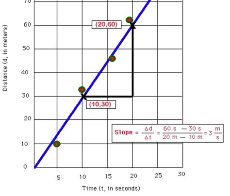
Table of Contents
Decoding the Slope: A Deep Dive into Position vs. Time Graphs
Understanding motion is fundamental to physics, and a powerful tool for visualizing and analyzing motion is the position-time graph. This graph plots an object's position on the y-axis against the time elapsed on the x-axis. The most crucial aspect of interpreting these graphs lies in understanding the slope of the position vs. time graph, which reveals crucial information about the object's velocity. This article will explore this concept in detail, covering various scenarios and providing practical examples.
What Does the Slope of a Position-Time Graph Represent?
The slope of a position-time graph represents the velocity of the object. This is a fundamental concept in kinematics, the study of motion. Remember that velocity is a vector quantity, meaning it has both magnitude (speed) and direction. Therefore, the slope's sign indicates the direction of motion.
-
Positive Slope: A positive slope indicates that the object is moving in the positive direction (typically considered to the right or upwards). As time increases, the position also increases.
-
Negative Slope: A negative slope indicates that the object is moving in the negative direction (typically considered to the left or downwards). As time increases, the position decreases.
-
Zero Slope: A zero slope indicates that the object is at rest; its position is not changing with respect to time. The object is stationary.
Calculating Velocity from the Slope
Calculating the velocity from a position-time graph is straightforward. The slope is calculated using the standard formula:
Slope = (Change in Position) / (Change in Time) = Δy / Δx = (y₂ - y₁) / (x₂ - x₁)
Where:
- y₂ and y₁ are the final and initial positions, respectively.
- x₂ and x₁ are the final and initial times, respectively.
This calculation gives you the average velocity over the time interval considered. To find the instantaneous velocity at a specific point, you would need to find the slope of the tangent line at that point.
Interpreting Different Types of Position-Time Graphs
Position-time graphs can take various forms, each representing a different type of motion. Let's explore some common scenarios:
1. Constant Velocity Motion
A graph representing constant velocity motion will be a straight line. The slope of this line will be constant, indicating a constant velocity. The steeper the line, the greater the magnitude of the velocity.
- Example: A car traveling at a steady 60 km/h on a straight highway will have a position-time graph showing a straight line with a positive slope.
2. Accelerated Motion
Accelerated motion is represented by a curved line on a position-time graph. The slope of the curve changes constantly, reflecting the changing velocity.
- Example: A ball thrown vertically upwards will initially have a positive slope (positive velocity), then the slope will decrease to zero at the highest point (zero velocity), and finally become negative as it falls back down (negative velocity).
3. Non-Uniform Acceleration
In cases of non-uniform acceleration, the position-time graph will be a more complex curve. The slope will continuously change, reflecting the continuously changing velocity and acceleration. This could represent, for example, a car accelerating at a rate that varies over time.
4. Stationary Object
A horizontal straight line on a position-time graph indicates a stationary object. The slope is zero, signifying zero velocity. The object's position remains constant over time.
Advanced Concepts and Applications
1. Instantaneous Velocity vs. Average Velocity
The slope of a secant line on a position-time graph represents the average velocity over a given time interval. However, the slope of a tangent line at a specific point represents the instantaneous velocity at that precise moment. This distinction is crucial for analyzing motion where velocity changes continuously.
2. Displacement vs. Distance
It's important to remember that the position-time graph shows displacement, not necessarily the total distance traveled. Displacement is the change in position from the starting point, while distance is the total length of the path traveled. For example, if an object moves 5 meters forward and then 2 meters backward, its displacement is 3 meters, but its distance traveled is 7 meters. The position-time graph only reflects the displacement.
3. Using Calculus for More Complex Scenarios
For more complex scenarios, such as motion described by non-linear functions, calculus becomes essential. The derivative of the position function with respect to time gives the velocity function, and the slope of the position-time graph at any point is the instantaneous velocity at that point, as defined by the derivative. Similarly, the second derivative provides the acceleration.
4. Real-world applications
Understanding position-time graphs and their slopes has widespread applications in various fields:
-
Physics: Analyzing projectile motion, understanding simple harmonic motion, and studying the motion of celestial bodies.
-
Engineering: Designing and optimizing the performance of vehicles, robotics, and control systems.
-
Sports science: Analyzing the performance of athletes, optimizing training programs, and understanding movement patterns.
-
Traffic analysis: Studying traffic flow, identifying bottlenecks, and improving traffic management strategies.
Practical Exercises and Examples
To solidify your understanding, try these exercises:
Exercise 1:
Sketch a position-time graph for an object that:
- Starts at rest at position 0 meters.
- Accelerates uniformly for 5 seconds.
- Moves at a constant velocity for 10 seconds.
- Decelerates uniformly to a stop over 5 seconds.
Exercise 2:
Given a position-time graph with the following points: (1s, 2m), (3s, 6m), (5s, 10m), determine the average velocity between:
- 1s and 3s.
- 3s and 5s.
- 1s and 5s.
Exercise 3:
Describe the motion represented by a position-time graph that is:
- A straight line with a negative slope.
- A parabolic curve opening upwards.
- A horizontal line.
By working through these exercises and exploring the various scenarios discussed above, you'll develop a strong grasp of how to interpret position-time graphs and extract meaningful information about the motion of an object. Remember, the key lies in understanding that the slope of the position-time graph is the velocity, and this principle underpins a large part of kinematics and its applications. Mastering this concept will significantly improve your ability to analyze and understand motion in various contexts.
Latest Posts
Latest Posts
-
General Chemistry Principles And Modern Applications
Mar 23, 2025
-
Is Viscosity A Chemical Or Physical Property
Mar 23, 2025
-
First Derivative And Second Derivative Test
Mar 23, 2025
-
How To Factor A Trinomial With A Leading Coefficient
Mar 23, 2025
-
Lanthanides And Actinides On The Periodic Table
Mar 23, 2025
Related Post
Thank you for visiting our website which covers about Slope Of Position Vs Time Graph . We hope the information provided has been useful to you. Feel free to contact us if you have any questions or need further assistance. See you next time and don't miss to bookmark.
