What Is The Mle Of Geometric
Muz Play
Mar 17, 2025 · 6 min read
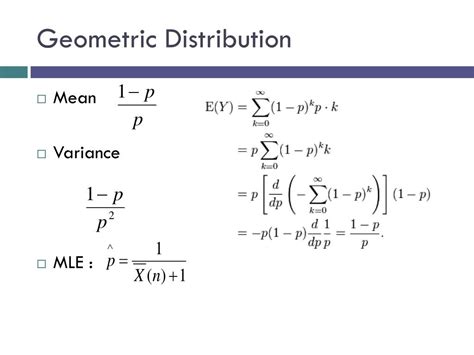
Table of Contents
What is the MLE of Geometric Distribution? A Comprehensive Guide
The geometric distribution is a fundamental concept in probability and statistics, frequently used to model the number of trials needed to achieve the first success in a sequence of independent Bernoulli trials. Understanding its properties, especially its Maximum Likelihood Estimator (MLE), is crucial for various applications ranging from reliability engineering to clinical trials. This comprehensive guide will delve deep into the geometric distribution, focusing on deriving and interpreting its MLE.
Understanding the Geometric Distribution
The geometric distribution describes the probability of observing the first success on the kth trial in a series of independent Bernoulli trials, each with a constant probability of success, denoted as p. This implies that the probability of failure is (1-p) = q.
The probability mass function (PMF) of a geometric distribution is given by:
P(X = k) = (1-p)^(k-1) * p, where:
- X represents the random variable denoting the number of trials until the first success.
- k is the number of trials until the first success (k = 1, 2, 3...).
- p is the probability of success in a single trial (0 < p ≤ 1).
There are two common variations of the geometric distribution:
- The number of failures before the first success: This formulation defines the random variable as the number of failures before the first success. The PMF in this case is: P(X = k) = (1-p)^k * p. Note that here, k can be 0, 1, 2...
This subtle difference can significantly impact the MLE derivation. We will primarily focus on the first definition (number of trials until the first success) in this guide, but will highlight the differences when relevant.
Deriving the MLE for the Geometric Distribution (Number of Trials Until First Success)
The Maximum Likelihood Estimation (MLE) method aims to find the value of the parameter (p in this case) that maximizes the likelihood function. The likelihood function, L(p), represents the probability of observing the sample data given a specific value of p.
Let's assume we have a random sample of size n from a geometric distribution: x₁, x₂, ..., xₙ. The likelihood function is the product of the individual probabilities:
L(p) = Πᵢ₌₁ⁿ [(1-p)^(xi-1) * p]
To simplify this expression, we can use logarithms. Taking the natural logarithm of the likelihood function (log-likelihood) doesn't change the location of the maximum, and it simplifies calculations considerably:
ln L(p) = Σᵢ₌₁ⁿ [ (xi - 1)ln(1-p) + ln(p) ]
To find the MLE, we take the derivative of the log-likelihood function with respect to p, set it to zero, and solve for p:
d(ln L(p))/dp = Σᵢ₌₁ⁿ [ -(xi - 1)/(1-p) + 1/p ] = 0
This equation simplifies to:
Σᵢ₌₁ⁿ [ -(xi - 1)/(1-p) + 1/p ] = 0
Solving for p, we get:
p = 1 / ( Σᵢ₌₁ⁿ xi / n )
Therefore, the MLE for the probability of success (p) in a geometric distribution (number of trials until the first success) is:
p̂ = n / Σᵢ₌₁ⁿ xi
This elegantly simple result shows that the MLE of p is simply the reciprocal of the sample mean. This intuitive result makes sense: a higher sample mean indicates a lower probability of success, and vice-versa.
Deriving the MLE for the Geometric Distribution (Number of Failures Before First Success)
For the alternative definition (number of failures before the first success), the likelihood function changes slightly:
L(p) = Πᵢ₌₁ⁿ [(1-p)^(xi) * p]
Following the same steps as above (taking the log-likelihood and finding its derivative), the MLE for p becomes:
p̂ = n / (Σᵢ₌₁ⁿ xi + n)
Notice the crucial difference: the denominator now includes n, accounting for the fact that we are considering the number of failures rather than the total number of trials.
Properties and Interpretation of the MLE for the Geometric Distribution
The MLE for the geometric distribution possesses several desirable statistical properties:
- Consistency: As the sample size (n) increases, the MLE converges to the true value of p.
- Asymptotic Normality: For large sample sizes, the MLE is approximately normally distributed with mean p and variance p(1-p)/n. This property is invaluable for constructing confidence intervals and hypothesis tests.
- Efficiency: The MLE is an efficient estimator, meaning it has the smallest possible variance among all unbiased estimators.
The interpretation of the MLE is straightforward: it provides the most likely value of the probability of success (p) based on the observed data. For instance, if we observe a sample mean of 5 trials until the first success, the MLE estimate of p would be 1/5 = 0.2. This suggests that the true probability of success in each trial is likely around 20%.
Applications of the Geometric Distribution and its MLE
The geometric distribution and its MLE find applications in various fields:
- Reliability Engineering: Modeling the time until failure of a component. The MLE can be used to estimate the probability of failure in a given time interval.
- Quality Control: Estimating the probability of a defective item in a production process. The MLE can be used to assess the effectiveness of quality control measures.
- Clinical Trials: Determining the probability of a successful treatment. The MLE can be used to assess the efficacy of a new drug or therapy.
- Sports Analytics: Analyzing the probability of a player scoring a goal or making a successful shot. The MLE can be used to evaluate player performance and predict future outcomes.
- Queuing Theory: Modeling the number of customers served before a server becomes idle. The MLE allows to estimate the service rate.
Bias and Variance of the MLE
While the MLE is unbiased for large sample sizes, it's slightly biased for small samples. This bias diminishes as n increases. The variance of the MLE, p(1-p)/n, also decreases as n increases, reflecting the improved accuracy of the estimate with more data.
Confidence Intervals for the MLE
Given the asymptotic normality of the MLE, we can construct confidence intervals for p. For a (1-α) confidence interval:
p̂ ± Z_(α/2) * sqrt[ p̂(1-p̂)/n ]
Where Z_(α/2) is the critical value from the standard normal distribution corresponding to the desired confidence level.
Hypothesis Testing with the MLE
We can perform hypothesis tests on the parameter p using the MLE. For example, we might test whether the probability of success is significantly different from a specific value (e.g., testing H₀: p = 0.5 vs. H₁: p ≠ 0.5). This can be done using a z-test based on the asymptotic normality of the MLE.
Conclusion
The MLE for the geometric distribution provides a powerful and efficient method for estimating the probability of success based on observed data. Its relatively simple derivation and intuitive interpretation make it a valuable tool in various applications across diverse fields. Understanding its properties, including its asymptotic normality, allows for the construction of confidence intervals and hypothesis tests, further strengthening its usefulness in statistical inference. While minor bias might be present in small samples, the MLE’s consistency and efficiency make it a preferred estimator for the geometric distribution’s parameter. Remember to choose the appropriate formulation of the geometric distribution (number of trials or number of failures) depending on the specific problem you are addressing.
Latest Posts
Latest Posts
-
Minerals Are Formed By The Process Of
Mar 17, 2025
-
M7 9 3 Perimeters And Areas Of Comp Fig
Mar 17, 2025
-
Investigation Mitosis And Cancer Answer Key
Mar 17, 2025
-
Where Is Halogens On The Periodic Table
Mar 17, 2025
-
Function Of A Stage On A Microscope
Mar 17, 2025
Related Post
Thank you for visiting our website which covers about What Is The Mle Of Geometric . We hope the information provided has been useful to you. Feel free to contact us if you have any questions or need further assistance. See you next time and don't miss to bookmark.
