Construct The Confidence Interval For The Population Mean Μ
Muz Play
Mar 25, 2025 · 6 min read
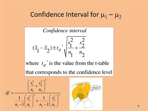
Table of Contents
Constructing the Confidence Interval for the Population Mean (μ)
Understanding and constructing confidence intervals for the population mean (μ) is a cornerstone of inferential statistics. It allows us to estimate the range within which the true population mean likely lies, based on a sample of data. This article will comprehensively guide you through the process, covering various scenarios and considerations. We'll delve into the theoretical underpinnings, practical applications, and the interpretation of results, equipping you with the knowledge to confidently utilize this powerful statistical tool.
Understanding Confidence Intervals
Before diving into the construction process, let's clarify the core concept. A confidence interval provides a range of plausible values for a population parameter (in this case, the mean μ). It's expressed as a percentage, commonly 95% or 99%, representing the confidence level. This confidence level signifies the long-run proportion of times that the constructed interval will contain the true population mean.
Key Components of a Confidence Interval:
- Point Estimate: This is the sample mean (x̄), calculated from your sample data. It serves as the best single guess for the population mean.
- Margin of Error: This accounts for the uncertainty inherent in using a sample to estimate the population mean. A larger margin of error indicates greater uncertainty.
- Confidence Level: This expresses the probability that the interval contains the true population mean. A higher confidence level leads to a wider interval.
The general formula for a confidence interval is:
Point Estimate ± Margin of Error
In the context of the population mean:
x̄ ± Margin of Error
Constructing Confidence Intervals: Different Scenarios
The method for constructing a confidence interval depends on several factors, primarily the sample size (n) and whether the population standard deviation (σ) is known.
Scenario 1: Population Standard Deviation (σ) Known, Large Sample (n ≥ 30)
When the population standard deviation is known and the sample size is large (generally considered n ≥ 30), the Central Limit Theorem allows us to use the z-distribution to construct the confidence interval. The formula is:
x̄ ± z(σ/√n)*
Where:
- x̄ is the sample mean.
- z is the z-score corresponding to the desired confidence level (e.g., 1.96 for a 95% confidence level, 2.58 for a 99% confidence level). You can find these values in a standard z-table or use statistical software.
- σ is the population standard deviation.
- n is the sample size.
Example:
Suppose we have a sample of 100 light bulbs (n=100), with a mean lifespan of 800 hours (x̄=800). We know the population standard deviation is 50 hours (σ=50). To construct a 95% confidence interval:
- Find the z-score for a 95% confidence level: z = 1.96
- Calculate the margin of error: 1.96 * (50/√100) = 9.8
- Construct the confidence interval: 800 ± 9.8 = (790.2, 809.8)
Therefore, we are 95% confident that the true mean lifespan of all light bulbs lies between 790.2 and 809.8 hours.
Scenario 2: Population Standard Deviation (σ) Unknown, Large Sample (n ≥ 30)
When the population standard deviation is unknown but the sample size is large (n ≥ 30), we estimate σ using the sample standard deviation (s). The Central Limit Theorem still applies, and we use the t-distribution instead of the z-distribution. The formula becomes:
x̄ ± t(s/√n)*
Where:
- x̄ is the sample mean.
- t is the t-score corresponding to the desired confidence level and degrees of freedom (df = n - 1). You'll need a t-table or statistical software to find this value.
- s is the sample standard deviation.
- n is the sample size.
Example:
Let's say we have a sample of 50 students (n=50) with an average test score of 75 (x̄=75) and a sample standard deviation of 10 (s=10). To construct a 99% confidence interval:
- Determine the degrees of freedom: df = 50 - 1 = 49
- Find the t-score for a 99% confidence level and 49 degrees of freedom: t ≈ 2.68 (using a t-table or software)
- Calculate the margin of error: 2.68 * (10/√50) ≈ 3.79
- Construct the confidence interval: 75 ± 3.79 = (71.21, 78.79)
We are 99% confident that the true average test score for all students lies between 71.21 and 78.79.
Scenario 3: Population Standard Deviation (σ) Unknown, Small Sample (n < 30)
When both the population standard deviation is unknown and the sample size is small (n < 30), the t-distribution is essential. The formula remains the same as in Scenario 2:
x̄ ± t(s/√n)*
However, the choice of the t-score is crucial. The smaller the sample size, the larger the t-score for the same confidence level, reflecting the increased uncertainty associated with smaller samples. Again, use a t-table or statistical software to find the appropriate t-score based on your degrees of freedom (n-1) and desired confidence level.
Scenario 4: Using Statistical Software
Statistical software packages like R, SPSS, Python (with libraries like SciPy and Statsmodels), and Excel make constructing confidence intervals significantly easier. These tools automate the calculations and provide the confidence interval directly, along with other relevant statistics. They handle the complexities of different distributions and sample sizes seamlessly.
Interpreting Confidence Intervals
The interpretation of a confidence interval is crucial. A 95% confidence interval, for instance, does not mean there is a 95% probability that the true population mean falls within the calculated interval. Instead, it means that if we were to repeatedly take samples and construct confidence intervals using the same method, 95% of those intervals would contain the true population mean.
Factors Affecting Confidence Interval Width
Several factors influence the width of a confidence interval:
- Sample Size (n): Larger samples lead to narrower intervals, reflecting reduced uncertainty.
- Confidence Level: Higher confidence levels (e.g., 99% vs. 95%) result in wider intervals. Greater certainty requires a broader range.
- Population Standard Deviation (σ or s): Larger standard deviations imply greater variability in the data, leading to wider intervals.
Common Mistakes to Avoid
- Misinterpreting the Confidence Level: Remember that the confidence level refers to the long-run frequency of intervals containing the true mean, not the probability that a specific interval contains the true mean.
- Ignoring Assumptions: The validity of the methods described depends on assumptions about the data (e.g., normality for small samples). Violating these assumptions can lead to inaccurate results.
- Using the Wrong Distribution: Choosing the wrong distribution (z vs. t) significantly impacts the interval width and accuracy.
Conclusion
Constructing confidence intervals for the population mean is a fundamental statistical technique. Understanding the different scenarios, applying the correct formulas, and correctly interpreting the results are essential for drawing valid inferences from sample data. Utilizing statistical software can streamline the process and ensure accuracy, particularly for complex situations. By mastering this technique, you gain a powerful tool for making informed decisions based on data analysis. Remember to always consider the context of your data, potential biases, and limitations when interpreting your confidence intervals.
Latest Posts
Latest Posts
-
Types Of Chemical Reactions Lab Answer Key
Mar 26, 2025
-
Double Angle And Half Angle Identities Worksheet
Mar 26, 2025
-
Periodic Table With Protons And Neutrons
Mar 26, 2025
-
The Movement Of Materials From High To Low Concentration
Mar 26, 2025
-
Elements With Similar Chemical Properties Are Found
Mar 26, 2025
Related Post
Thank you for visiting our website which covers about Construct The Confidence Interval For The Population Mean Μ . We hope the information provided has been useful to you. Feel free to contact us if you have any questions or need further assistance. See you next time and don't miss to bookmark.
