Turbulent Channel Flow Near Wall Velocity Profile
Muz Play
Mar 29, 2025 · 6 min read
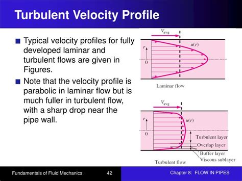
Table of Contents
Turbulent Channel Flow Near-Wall Velocity Profile: A Deep Dive
Turbulent channel flow, a fundamental problem in fluid mechanics, presents a fascinating and complex challenge. Understanding the velocity profile, especially near the wall, is crucial for various engineering applications, from designing efficient heat exchangers to predicting drag in pipelines. This article delves deep into the intricacies of the near-wall velocity profile in turbulent channel flow, exploring the governing physics, empirical laws, and advanced modeling techniques.
Understanding the Basics: Laminar vs. Turbulent Flow
Before diving into the complexities of turbulent channel flow, let's establish a baseline understanding of laminar and turbulent flow regimes. Laminar flow is characterized by smooth, ordered fluid motion, where fluid particles move in parallel layers. Turbulent flow, on the other hand, is characterized by chaotic, irregular motion with swirling eddies and fluctuations in velocity. This transition from laminar to turbulent flow depends on the Reynolds number (Re), a dimensionless quantity representing the ratio of inertial forces to viscous forces. For channel flow, a critical Reynolds number (typically around 2300) marks the transition.
The Near-Wall Region: A Realm of Complex Interactions
The near-wall region in turbulent channel flow is a zone of intense shear and complex interactions between viscous and turbulent effects. It's typically divided into several distinct layers based on the dominant physical mechanisms:
1. Viscous Sublayer: The Domain of Viscosity
This innermost layer, closest to the wall, is dominated by viscous forces. The velocity profile is almost linear and follows a relationship closely approximated by:
u⁺ = y⁺
where:
- u⁺ = u/uτ is the dimensionless velocity, with u being the streamwise velocity and uτ the friction velocity (a measure of the shear stress at the wall).
- y⁺ = yuτ/ν is the dimensionless wall distance, with y being the distance from the wall and ν the kinematic viscosity.
This linear relationship holds for y⁺ < 5 approximately. Within this region, the flow is primarily laminar, despite being embedded within a turbulent flow field.
2. Buffer Layer: A Transitional Zone
The buffer layer sits between the viscous sublayer and the logarithmic layer. It's a transition zone where both viscous and turbulent effects are significant. The velocity profile in this layer is neither purely linear nor purely logarithmic. It's characterized by a steeper slope than the viscous sublayer and a gradual transition to the logarithmic profile. The buffer layer typically spans 5 < y⁺ < 30. Predicting the velocity profile in this region is challenging and often requires sophisticated turbulence models.
3. Logarithmic Layer: The Turbulent Core
The logarithmic layer, extending from y⁺ ≈ 30 to y⁺ ≈ 0.2Reδ (where Reδ is the Reynolds number based on the channel half-width δ), is characterized by a logarithmic velocity profile. This is often expressed as:
u⁺ = (1/κ)ln(y⁺) + B
where:
- κ is the von Kármán constant (approximately 0.41) – a dimensionless empirical constant reflecting the turbulent mixing properties.
- B is another empirical constant (typically around 5).
This logarithmic law represents the equilibrium state between the production and dissipation of turbulent kinetic energy. In this region, the flow is fully turbulent, with large-scale eddies dominating the flow structure.
4. Outer Layer (Wake Region): The Influence of the Centerline
Beyond the logarithmic layer, the outer layer, or wake region, extends towards the center of the channel. In this region, the velocity profile deviates from the logarithmic law, influenced by the centerline velocity and the overall flow structure. The precise description of the velocity profile in this region is complex and requires more advanced modeling techniques.
Empirical Laws and Their Limitations
While the logarithmic law provides a good approximation for the velocity profile in the logarithmic layer, it's essential to acknowledge its limitations. These empirical laws are based on experimental observations and statistical averaging, and they don't capture the instantaneous, fluctuating nature of turbulent flow. Furthermore, the constants κ and B are not truly universal and can vary slightly depending on the Reynolds number and experimental setup.
Advanced Modeling Techniques: Computational Fluid Dynamics (CFD)
Advanced numerical techniques, such as Computational Fluid Dynamics (CFD), are essential for accurate prediction of the near-wall velocity profile in turbulent channel flow. CFD employs sophisticated turbulence models to resolve the complex interactions and fluctuations within the flow. These models range from simple algebraic models to advanced Reynolds-averaged Navier-Stokes (RANS) models and large eddy simulation (LES) approaches.
Reynolds-Averaged Navier-Stokes (RANS) Models
RANS models decompose the flow variables into mean and fluctuating components and solve for the mean flow characteristics. Common RANS models include the k-ε model and the k-ω SST model. These models require near-wall treatments to accurately capture the velocity profile in the near-wall region. Wall functions are often employed to bridge the gap between the resolved flow and the viscous sublayer.
Large Eddy Simulation (LES)
LES resolves the large-scale turbulent structures directly, while modeling the small-scale structures using subgrid-scale models. LES offers a higher fidelity representation of turbulent flows compared to RANS, but it's computationally more expensive. It's particularly suitable for resolving the intricate details of the near-wall region.
Direct Numerical Simulation (DNS)
DNS directly solves the Navier-Stokes equations without any turbulence modeling. This provides the most accurate representation of the flow, but it's computationally extremely expensive and limited to low Reynolds numbers. It plays a crucial role in validating and improving turbulence models.
Applications and Significance
Understanding the near-wall velocity profile in turbulent channel flow has far-reaching implications across various engineering disciplines:
- Heat Transfer: Accurate prediction of the velocity profile is crucial for designing efficient heat exchangers and other thermal systems. The near-wall region plays a dominant role in heat transfer due to its high shear rates.
- Drag Reduction: Minimizing drag in pipelines and other flow systems is vital for energy efficiency. Understanding the near-wall flow characteristics allows for the development of drag-reducing strategies.
- Aerodynamics: The near-wall flow significantly affects the aerodynamic performance of aircraft and other vehicles. Accurate modeling is essential for designing efficient and stable aerodynamic surfaces.
- Environmental Engineering: Turbulent channel flow plays a role in various environmental processes, such as river flows and pollutant dispersion. Understanding the near-wall velocity profile aids in modeling these processes and managing environmental impacts.
Conclusion: Ongoing Research and Future Directions
The study of turbulent channel flow near-wall velocity profiles remains a vibrant area of research. While significant progress has been made in understanding the governing physics and developing advanced modeling techniques, many challenges persist. Further research is needed to improve turbulence models, particularly in the buffer layer, and to develop more efficient numerical methods for simulating complex turbulent flows. The development of more accurate and robust models will have significant implications for numerous engineering applications and our fundamental understanding of turbulent flows. The continued exploration of this fascinating field promises exciting advancements in our ability to predict and control turbulent flows.
Latest Posts
Latest Posts
-
Political Map Of North Africa And Southwest Asia
Mar 31, 2025
-
Work Is The Integral Of Force
Mar 31, 2025
-
Is Water A Reactant Or Product
Mar 31, 2025
-
Four Ways To Represent A Function
Mar 31, 2025
-
What Is The Functional Unit Of Heredity
Mar 31, 2025
Related Post
Thank you for visiting our website which covers about Turbulent Channel Flow Near Wall Velocity Profile . We hope the information provided has been useful to you. Feel free to contact us if you have any questions or need further assistance. See you next time and don't miss to bookmark.
