Formula For Motion With Constant Acceleration
Muz Play
Mar 24, 2025 · 6 min read
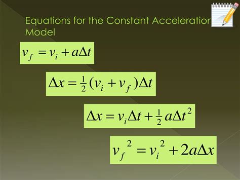
Table of Contents
The Formula for Motion with Constant Acceleration: A Comprehensive Guide
Understanding motion is fundamental to physics. Whether it's analyzing the trajectory of a projectile, predicting the speed of a car accelerating down a highway, or designing a new rollercoaster, the ability to describe and predict motion is crucial. This article delves deep into the equations of motion for objects experiencing constant acceleration, exploring their derivations, applications, and practical implications.
What is Constant Acceleration?
Before diving into the formulas, let's define our key term: constant acceleration. Acceleration, in simple terms, is the rate at which an object's velocity changes over time. Constant acceleration means this rate of change remains uniform; it doesn't speed up or slow down its increase or decrease in speed. This is an idealization, as in the real world, friction and other forces often lead to non-constant acceleration. However, the constant acceleration model is a powerful tool for understanding and approximating many real-world scenarios.
The Key Equations of Motion (SUVAT Equations)
The equations of motion for constant acceleration are often referred to as the SUVAT equations. SUVAT is an acronym representing the five key variables involved:
- s: Displacement (often denoted as Δx or Δy depending on the direction of motion) - the change in position of the object. Measured in meters (m).
- u: Initial velocity – the velocity of the object at the beginning of the considered time interval. Measured in meters per second (m/s).
- v: Final velocity – the velocity of the object at the end of the considered time interval. Measured in meters per second (m/s).
- a: Acceleration – the constant rate of change of velocity. Measured in meters per second squared (m/s²).
- t: Time – the duration of the motion being considered. Measured in seconds (s).
These five variables are related through four fundamental equations:
1. v = u + at
This equation directly relates final velocity (v) to initial velocity (u), acceleration (a), and time (t). It states that the final velocity is the initial velocity plus the change in velocity due to acceleration over time.
Derivation: Acceleration is defined as the change in velocity divided by the change in time: a = (v - u) / t. Rearranging this equation gives us v = u + at.
2. s = ut + (1/2)at²
This equation calculates the displacement (s) based on initial velocity (u), acceleration (a), and time (t). It shows that displacement is the sum of the distance covered at initial velocity and the additional distance covered due to acceleration.
Derivation: This equation can be derived using calculus or through a graphical interpretation of velocity-time graphs. The displacement is the area under the velocity-time graph, which is a trapezium for constant acceleration. The area of a trapezium is given by (1/2)(sum of parallel sides)(height), leading to s = ut + (1/2)at².
3. v² = u² + 2as
This equation links final velocity (v) to initial velocity (u), acceleration (a), and displacement (s). It eliminates time (t) as a variable, making it useful when time isn't explicitly given.
Derivation: This equation can be derived by eliminating 't' from equations 1 and 2. Solve equation 1 for t (t = (v-u)/a) and substitute it into equation 2. After some algebraic manipulation, you'll arrive at v² = u² + 2as.
4. s = [(u + v)/2]t
This equation calculates the displacement (s) using the average velocity [(u+v)/2] and the time (t). It assumes a constant acceleration. The average velocity is used because the velocity changes linearly.
Derivation: This equation can be derived directly from the graphical interpretation of the velocity-time graph. The average velocity is simply the average of the initial and final velocities, and the area under the graph (displacement) is the average velocity multiplied by the time.
Applying the Equations: Worked Examples
Let's solidify our understanding with some worked examples:
Example 1: A car accelerates from rest (u=0 m/s) at a constant rate of 2 m/s² for 5 seconds. What is its final velocity (v) and the distance (s) it travels?
- Given: u = 0 m/s, a = 2 m/s², t = 5 s
- Find: v, s
- Equation 1: v = u + at = 0 + (2)(5) = 10 m/s
- Equation 2: s = ut + (1/2)at² = (0)(5) + (1/2)(2)(5)² = 25 m
Therefore, the car's final velocity is 10 m/s, and it travels 25 meters.
Example 2: A ball is thrown vertically upwards with an initial velocity of 20 m/s. Ignoring air resistance, and assuming a constant downward acceleration due to gravity (g ≈ 9.8 m/s²), what is the maximum height the ball reaches?
- Given: u = 20 m/s, a = -9.8 m/s² (negative because gravity acts downwards), v = 0 m/s (at the maximum height, velocity is momentarily zero).
- Find: s (maximum height)
- Equation 3: v² = u² + 2as => 0 = 20² + 2(-9.8)s => s = 20²/19.6 ≈ 20.4 m
The ball reaches a maximum height of approximately 20.4 meters.
Example 3: A train decelerates uniformly from 30 m/s to 10 m/s over a distance of 100m. What is its acceleration?
- Given: u = 30 m/s, v = 10 m/s, s = 100 m
- Find: a
- Equation 3: v² = u² + 2as => 10² = 30² + 2a(100) => a = (10² - 30²)/(200) = -4 m/s²
The train's acceleration is -4 m/s², indicating deceleration.
Limitations and Extensions of the Model
It's crucial to remember that the SUVAT equations are based on the assumption of constant acceleration. In reality, this is often an approximation. Factors like air resistance, friction, and changing gravitational fields can lead to non-constant acceleration. For more complex scenarios, more advanced techniques like calculus-based approaches are necessary.
Furthermore, these equations are vector equations; they work in multiple dimensions. You need to consider the x and y components separately in a two-dimensional motion, where you would have separate equations for each direction. For projectile motion, for example, you will have a constant acceleration in the y-direction (gravity) and usually a constant zero acceleration in the x-direction (ignoring air resistance).
Applications in Real-World Scenarios
The equations of motion with constant acceleration have widespread applications in various fields:
- Engineering: Designing vehicles, launching rockets, and analyzing structural stability under dynamic loads.
- Sports Science: Analyzing the performance of athletes, optimizing training strategies, and understanding the mechanics of movement in sports.
- Robotics: Controlling the movement of robots, designing robotic arms, and programming autonomous navigation systems.
- Aerospace: Trajectory prediction, satellite control, and the design of aircraft and spacecraft.
- Physics: Understanding fundamental principles of motion, testing theories, and modeling physical phenomena.
Conclusion
The formulas for motion with constant acceleration are essential tools for understanding and predicting the motion of objects. While the assumption of constant acceleration is an idealization, these equations provide a powerful framework for analyzing a wide range of real-world scenarios. By understanding the derivations and applications of the SUVAT equations, you gain a deeper appreciation for the fundamental principles of kinematics and their importance across various scientific and engineering disciplines. Mastering these equations opens doors to solving many challenging problems related to motion and lays a solid foundation for further explorations into more complex dynamics. Remember to always carefully define your coordinate system, and consider the direction of your vectors (positive or negative), to accurately apply these equations.
Latest Posts
Latest Posts
-
Does Adding A Catalyst Increase The Rate Of Reaction
Mar 26, 2025
-
How To Calculate The Freezing Point Of A Solution
Mar 26, 2025
-
Chemical Equilibrium Le Chateliers Principle Lab Answers
Mar 26, 2025
-
Peroxisomes Got Their Name Because Hydrogen Peroxide Is
Mar 26, 2025
-
State Of Matter With Definite Shape And Volume
Mar 26, 2025
Related Post
Thank you for visiting our website which covers about Formula For Motion With Constant Acceleration . We hope the information provided has been useful to you. Feel free to contact us if you have any questions or need further assistance. See you next time and don't miss to bookmark.
