Laplace Equation In Spherical Polar Coordinates
Muz Play
Mar 17, 2025 · 5 min read
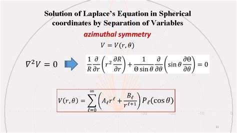
Table of Contents
Laplace Equation in Spherical Polar Coordinates: A Comprehensive Guide
The Laplace equation, a cornerstone of mathematical physics, describes steady-state phenomena where there are no sources or sinks. It finds applications in diverse fields, including electrostatics, fluid dynamics, heat transfer, and gravitational potential. While readily solved in Cartesian coordinates, its application in systems with inherent spherical symmetry necessitates its formulation in spherical polar coordinates. This article provides a comprehensive exploration of the Laplace equation in spherical polar coordinates, covering its derivation, solutions, and practical applications.
Understanding Spherical Polar Coordinates
Before delving into the Laplace equation itself, let's establish a firm grasp of spherical polar coordinates (ρ, θ, φ). These coordinates represent a point in three-dimensional space using:
- ρ (rho): The radial distance from the origin to the point. This is always non-negative (ρ ≥ 0).
- θ (theta): The polar angle, measured from the positive z-axis towards the point. It ranges from 0 to π radians (0 ≤ θ ≤ π).
- φ (phi): The azimuthal angle, measured from the positive x-axis in the xy-plane to the projection of the point onto the xy-plane. It ranges from 0 to 2π radians (0 ≤ φ ≤ 2π).
The transformation from Cartesian coordinates (x, y, z) to spherical polar coordinates is given by:
- x = ρ sin θ cos φ
- y = ρ sin θ sin φ
- z = ρ cos θ
The inverse transformation is:
- ρ = √(x² + y² + z²)
- θ = arccos(z/ρ)
- φ = arctan(y/x)
Deriving the Laplace Equation in Spherical Polar Coordinates
The Laplace equation in Cartesian coordinates is:
∇²u = ∂²u/∂x² + ∂²u/∂y² + ∂²u/∂z² = 0
To express this in spherical polar coordinates, we need to employ the chain rule and the transformation equations. This involves a significant amount of calculus, requiring careful application of partial derivatives. The resulting equation, after considerable algebraic manipulation, is:
∇²u = (1/ρ²) ∂/∂ρ (ρ² ∂u/∂ρ) + (1/(ρ² sin θ)) ∂/∂θ (sin θ ∂u/∂θ) + (1/(ρ² sin² θ)) ∂²u/∂φ² = 0
This is the Laplace equation in spherical polar coordinates. Its complexity highlights the advantage of using the appropriate coordinate system for a given problem.
Solving the Laplace Equation: Separation of Variables
Solving the Laplace equation directly is often challenging. A powerful technique is the method of separation of variables. This involves assuming a solution of the form:
u(ρ, θ, φ) = R(ρ)Θ(θ)Φ(φ)
Substituting this into the Laplace equation and dividing by u(ρ, θ, φ) leads to three separate ordinary differential equations, one for each variable:
-
Radial Equation (R(ρ)): This equation typically involves solving a second-order differential equation, often leading to solutions involving powers of ρ, spherical Bessel functions, or modified spherical Bessel functions, depending on the boundary conditions.
-
Polar Angle Equation (Θ(θ)): This equation is a second-order differential equation whose solutions are associated Legendre polynomials, Pₗₘ(cos θ), where l and m are separation constants.
-
Azimuthal Angle Equation (Φ(φ)): This equation is straightforward, yielding sinusoidal solutions of the form sin(mφ) or cos(mφ).
Legendre Polynomials and Associated Legendre Polynomials
The solutions to the polar angle equation, Θ(θ), are intimately linked to Legendre polynomials and their associated functions.
Legendre Polynomials, Pₗ(x): These are a set of orthogonal polynomials defined on the interval [-1, 1]. They are solutions to Legendre's differential equation and are crucial for solving the Laplace equation in spherical coordinates. The first few Legendre polynomials are:
- P₀(x) = 1
- P₁(x) = x
- P₂(x) = (3x² - 1)/2
- P₃(x) = (5x³ - 3x)/2
- ...and so on.
Associated Legendre Polynomials, Pₗₘ(x): These are generalizations of Legendre polynomials, incorporating the azimuthal quantum number, m. They are defined as:
Pₗₘ(x) = (1 - x²)^(|m|/2) d^|m|/dx^|m| Pₗ(x)
These polynomials are essential for handling the azimuthal dependence in the solution.
Spherical Harmonics
The product of the solutions to the polar angle and azimuthal angle equations forms the spherical harmonics, Yₗₘ(θ, φ):
Yₗₘ(θ, φ) = A Pₗₘ(cos θ) e^(±imφ)
where A is a normalization constant. Spherical harmonics form a complete orthonormal set of functions on the unit sphere, making them invaluable in various physical applications.
General Solution and Boundary Conditions
The general solution to the Laplace equation in spherical polar coordinates is a linear combination of the individual solutions:
u(ρ, θ, φ) = Σₗ Σₘ [Aₗₘρˡ + Bₗₘρ⁻⁽ˡ⁺¹⁾] Yₗₘ(θ, φ)
where Aₗₘ and Bₗₘ are constants determined by the boundary conditions of the specific problem. The specific values of these constants depend entirely on the physical context: the geometry of the system, the nature of the potential or field, and the values specified at the boundaries.
Applications of the Laplace Equation in Spherical Polar Coordinates
The Laplace equation in spherical polar coordinates finds numerous applications across various scientific disciplines. Here are a few prominent examples:
Electrostatics
The electrostatic potential, V, outside a charged sphere satisfies the Laplace equation. By solving this equation with appropriate boundary conditions, we can determine the potential at any point in space.
Fluid Dynamics
In fluid mechanics, the Laplace equation governs irrotational, incompressible fluid flow. This has significant implications in understanding phenomena like potential flow around submerged objects.
Heat Transfer
The temperature distribution in a spherical object with constant temperature boundaries can be modeled using the Laplace equation.
Gravitational Potential
The gravitational potential due to a spherically symmetric mass distribution satisfies the Laplace equation in the regions outside the mass distribution.
Conclusion
The Laplace equation in spherical polar coordinates presents a powerful tool for addressing physical problems with inherent spherical symmetry. While its solution requires a deeper understanding of differential equations and special functions like Legendre polynomials and spherical harmonics, the results provide crucial insights into a vast range of phenomena across physics and engineering. Mastering this mathematical framework is essential for tackling sophisticated problems in diverse scientific fields, opening the door to a deeper understanding of the natural world. Further study into specific boundary conditions and the application of numerical methods can lead to a more nuanced appreciation of the equation’s power and versatility.
Latest Posts
Latest Posts
-
How Much Nadh Does Glycolysis Produce
Mar 17, 2025
-
What Is A Principal Agent In Insurance
Mar 17, 2025
-
Strong And Weak Acids And Bases List
Mar 17, 2025
-
Absorption Spectrum Of Helium Largest Transition
Mar 17, 2025
-
List Of Equipments For Validation In Pharma And Biotech Industry
Mar 17, 2025
Related Post
Thank you for visiting our website which covers about Laplace Equation In Spherical Polar Coordinates . We hope the information provided has been useful to you. Feel free to contact us if you have any questions or need further assistance. See you next time and don't miss to bookmark.
